Weight-Tying: The Small, Gentle Read–Write Symmetry in Language Models

TL;DR — A language model at every step asks one simple question — given the numerical representation of the context so far, what is the probability of each vocabulary token being next? This writing unfolds that question cleanly: symbols first, forward & backward passes next, then the split of gradients that makes a single embedding table both reader and writer.

Flow (how to read this note)

1. State the single desideratum that drives everything.
2. Fix notation and the primitive objects we will manipulate.
3. Walk forward: from tokens to probabilities.
4. Walk backward: show the two distinct gradient paths into the embedding matrix and why they differ in character.
5. Give a per-position worked derivative so nothing like magic.
6. Read the consequences: symmetry, sparsity vs. density, and computational cost.

Prelude — the single desideratum

At each time step the model must compute a distribution over vocabulary tokens. Put plainly:

Given the numeric representation of the context so far, compute $p(\text{next token} = v)$ for every $v\in\{0,\dots,V-1\}$.

Everything that follows is a careful unpacking of how we represent the context, how the model turns that representation into logits and probabilities, and how gradients flow back into the same parameters that produced the representation.

Notation and primitives

We define the notation so the shapes and roles are obvious.

• $B$ — batch size (parallel independent sequences).
• $T$ — sequence length (tokens per sequence).
• $D$ — model hidden / embedding dimension.
• $V$ — vocabulary size.

Primitive tensors:

• $X_{\text{ids}}\in\{0,\dots,V-1\}^{B\times T}$: token indices after tokenization.
• $E\in\mathbb{R}^{V\times D}$: token embedding matrix; row $E_{v,:}$ is the vector for token $v$.
• $P\in\mathbb{R}^{T\times D}$: positional embeddings (or any positional encoding of length $T$).
• $X\in\mathbb{R}^{B\times T\times D}$: token vectors with position; for a sequence position $(b,t)$, $$X_{b,t,:} = E_{X_{\text{ids}_{b,t}},:} + P_{t,:}.$$
• $\mathcal{T}(\cdot)$: the transformer stack — a deterministic, differentiable function mapping $X\mapsto H$.
• $H=\mathcal{T}(X)\in\mathbb{R}^{B\times T\times D}$: final hidden states.
• Tied LM head: $W = E^\top\in\mathbb{R}^{D\times V}$. (Tying enforces the same space for read/write.)
• $b\in\mathbb{R}^V$: optional bias on logits.
• $\ell$: scalar loss (we use mean cross-entropy over batch and time).

These primitives suffice to write the forward and backward equations compactly and exactly.

Forward pass

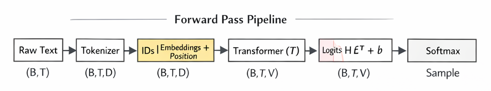
1. Embed + add position

   $$X_{b,t,:} = E_{X_{\text{ids}_{b,t}},:} + P_{t,:},\qquad X\in\mathbb{R}^{B\times T\times D}.$$

   Why: we need a dense vector representation for each token and a way to indicate position.

2. Transform

   $$H = \mathcal{T}(X),\qquad H\in\mathbb{R}^{B\times T\times D}.$$

   Why: the transformer composes attention and MLP layers to convert per-position inputs into context-aware representations.

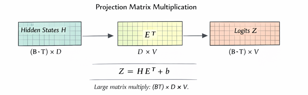
3. Logits via tied head

   $$Z = HE^\top + \mathbf{1}_{BT}b^\top,\qquad Z\in\mathbb{R}^{B\times T\times V}.$$

   Here $\mathbf{1}_{BT}$ indicates broadcasting the bias to every $(b,t)$ slice.

   Why: each hidden $h\in\mathbb{R}^D$ scores every vocabulary row by inner product with that row; tying uses the same rows that produced embeddings.

1. Softmax → probabilities

   $$p_{b,t,j}=\frac{\exp(Z_{b,t,j})}{\sum_{k=1}^V\exp(Z_{b,t,k})}.$$

2. Mean cross-entropy loss For targets $Y\in\{1,\dots,V\}^{B\times T}$,

   $$\ell = -\frac{1}{BT}\sum_{b=1}^B\sum_{t=1}^T \log p_{b,t,Y_{b,t}}.$$

These are the only forward equations required; they arise directly from the desideratum and the chosen primitives.

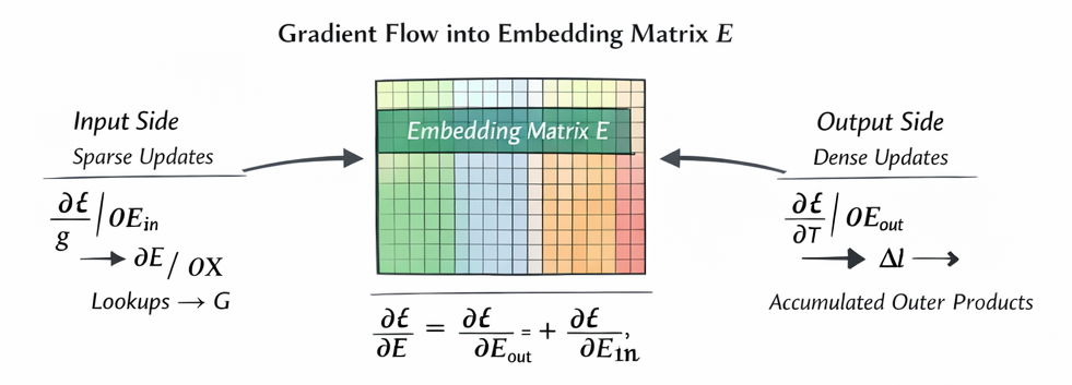
Backward pass — the two distinct contributions into $E$ (chain rule)

Because $E$ appears in two roles — as a lookup for inputs and as the transpose used to compute logits — the gradient $\frac{\partial \ell}{\partial E}$ decomposes into two additive pieces.

1. Immediate quantity from softmax + CE (logit residuals)

Define the logit residual tensor

This $\Delta\in\mathbb{R}^{B\times T\times V}$ is the primitive starting point for gradients flowing into both the head (output side) and back into $H$.

2. Output-side (projection) contribution — dense outer products

From $Z_{b,t,:} = H_{b,t,:}E^\top + b$ we obtain the gradient on $E$ coming from the head:

Concretely, for vocabulary row $v$,

Character: dense — typically every $v$ receives some (small) contribution because the softmax probabilities are dense.

3. Input-side (lookup) contribution — sparse accumulation

Backpropagating through the transformer yields gradients to its inputs:

Since $X_{b,t,:}=E_{X_{\text{ids}_{b,t}},:}+P_{t,:}$, the corresponding row of $E$ for the token $v=X_{\text{ids}_{b,t}}$ receives:

Character: sparse — only embedding rows for tokens present in the mini-batch are touched.

4. Total gradient on $E$

By linearity,

Pragmatically, frameworks accumulate both contributions into E.grad during a single backward pass.

A per-position worked derivative (so there is no mystery)

Fix a single position $(b,t)$. Let $h=H_{b,t,:}\in\mathbb{R}^D$, $z=Z_{b,t,:}\in\mathbb{R}^V$, and $y=Y_{b,t}$ the correct index.

• $p_j=\dfrac{e^{z_j}}{\sum_k e^{z_k}}$.
• $\dfrac{\partial \ell_{b,t}}{\partial z_j}=p_j-\mathbf{1}_{j=y}$.
• Output-side update for $E_{v,:}$ from this position: $$\dfrac{\partial \ell_{b,t}}{\partial E_{v,:}}^{\text{(out,pos)}} = (p_v-\mathbf{1}_{v=y})h^\top.$$
• Gradient into $h$ from the head: $$\dfrac{\partial \ell_{b,t}}{\partial h} = \sum_{v=1}^V (p_v-\mathbf{1}_{v=y})E_{v,:}^\top = E^\top (p - e_y).$$

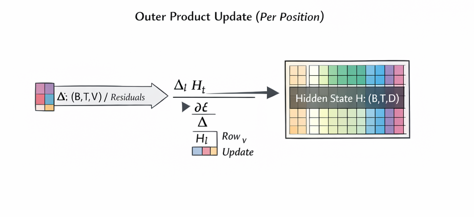
Summing these per-position contributions across $(b,t)$ recovers the tensor equations above. This shows how softmax residuals produce outer-product updates on $E$ and how they also feed back into the model via $h$.

Computational Accounting

Consider $B=4$, $T=128$, $D=4096$, $V=32{,}000$.

• $BT = 4\times128 = 512$.
• $(BT)\times D = 512\times4096 = 2{,}097{,}152$.
• Multiply by $V$: $2{,}097{,}152\times 32{,}000 = (2{,}097{,}152\times32)\times1000 = 67{,}108{,}864\times1000 = 67{,}108{,}864{,}000$.

So roughly $6.71\times 10^{10}$ multiply–accumulate operations are required for that single forward (or backward) pass through the head for the batch — a salutary reminder that the projection to vocabulary is often the dominant cost when $V$ is large.

Interpretation and Consequences

• Read–write symmetry. Tying $W=E^\top$ means the vector space used to read tokens (embedding lookup) is identical to the space used to write tokens (projection). This reduces parameter redundancy and aligns representation and generation semantics.
• Two distinct learning channels. An embedding row changes for two reasons: (i) its use as an input (sparse updates) and (ii) its role in predicting outputs (dense outer-product updates). Both matter, but they have very different computational and statistical character.
• Sparsity vs. density. Input-side updates touch only the rows present in the batch (sparse). Output-side updates touch all $V$ rows (dense) because softmax spreads probability mass over the vocabulary. This explains why the head can be a bottleneck in large-vocabulary models.
• Practical design choices. If $V$ is large, we can look towards techniques like: adaptive softmax, vocabulary culling, sampling-based losses, or token clustering, to reduce the dense cost while preserving predictive fidelity.

Closing Remark

The model reads by looking up embedding rows and writes by taking inner products with those same rows; tying them makes the read and write vocabularies identical, and backpropagation simply sums the sparse read-derived corrections with the dense write-derived outer-product corrections into one embedding table.